
Who has Championship Games with Larger Point Differentials and More Blowouts: NCAA or NFL?
Hey everyone! So, I wanted to share an analysis I performed on NCAA and NFL championship data.
To understand why I performed these analyses and made this notebook, it might help to have some context. So recently, my boss and I were discussing the 2020-2021 Super Bowl game. During our conversation, we had mentioned how surprised we were by the large point differential between the Tampa Bay Buccaneers and Kansas City Chiefs. Tampa Bay beat Kansas by 22 points, which to me seemed like a relatively large point differential for a professional football game. Now I will admit that I tend to watch more college than professional football, and thus have more experience with NCAA games. In the NCAA you can have large point differentials in games (i.e. Clemson beat Alabama by 28 points during the 2018-2019 year). This may be a result of particular conferences monopolizing better players/recruiting classes due to reputation.
All of this made me think that maybe the NCAA, on average, has larger point differentials in championship games than in professional football. Also, maybe it was possible the the NCAA had more blowout championship games than the NFL. So I wanted to test these hypotheses by gathering Super Bowl and NCAA championship data.
Load libraries
library(rvest) # For web scraping
library(tidyverse) # For Data cleaning
library(infer) #For Permutation testing
NFL Data
Web scrape Super Bowl data
NFL Data obtained from - https://www.pro-football-reference.com/super-bowl/
superbowl_df <- html_session('https://www.pro-football-reference.com/super-bowl/') %>%
  read_html() %>%
  html_node(xpath = '//*[@id="super_bowls"]') %>%
  html_table()

#Change column names
colnames(superbowl_df)[c(4, 6)] <- c('winning_team', 'losing_team')
head(superbowl_df)
Date <chr> | SB <chr> | Winner <chr> | winning_team <int> | Loser <chr> | ||
|---|---|---|---|---|---|---|
| 1 | Feb 7, 2021 | LV (55) | Tampa Bay Buccaneers | 31 | Kansas City Chiefs | |
| 2 | Feb 2, 2020 | LIV (54) | Kansas City Chiefs | 31 | San Francisco 49ers | |
| 3 | Feb 3, 2019 | LIII (53) | New England Patriots | 13 | Los Angeles Rams | |
| 4 | Feb 4, 2018 | LII (52) | Philadelphia Eagles | 41 | New England Patriots | |
| 5 | Feb 5, 2017 | LI (51) | New England Patriots | 34 | Atlanta Falcons | |
| 6 | Feb 7, 2016 | 50 | Denver Broncos | 24 | Carolina Panthers |
Filter data and calculate point differentials for Super Bowl
Please note that I will only be looking at data from 1990 to 2019
superbowl_filtered <- superbowl_df %>%
  mutate(year = as.integer(str_extract_all(Date, "[0-9]{4}")), point_differential =  winning_team - losing_team) %>%
  filter(year >= 1990 & year <= 2019) %>%
  select(year, point_differential)
Calculate descriptive statistics
summary(superbowl_filtered$point_differential)
   Min. 1st Qu.  Median    Mean 3rd Qu.    Max.
   1.00    4.00   10.00   12.80   14.75   45.00
NCAA Data
Web scrape NCAA football National championship data
NCAA Data obtained from - http://championshiphistory.com/ncaafootball.php
NCAA_df <- html_session('http://championshiphistory.com/ncaafootball.php') %>%
  read_html() %>%
  html_node(xpath = '//*[@id="tablesorter-demo"]') %>%
  html_table(fill = T)

NCAA_df <- na.omit(NCAA_df)
head(NCAA_df)
Year <int> | Era <chr> | #1 CollegeTeam <chr> | RunnerUp <chr> | Championship Score <chr> | ||
|---|---|---|---|---|---|---|
| 1 | 2019 | CFP | LSU Tigers | Clemson | 42-25 | |
| 3 | 2018 | CFP | Clemson | Alabama | 44-16 | |
| 5 | 2017 | CFP | Alabama | Georgia | 26-23 | |
| 7 | 2016 | CFP | Clemson | Alabama | 35-31 | |
| 9 | 2015 | CFP | Alabama | Clemson | 45-40 | |
| 11 | 2014 | CFP | Ohio State | Oregon | 42-20 |
Parse out championship scores for NCAA
# Calculate number of rows in NCAA data frame
num_games <- nrow(NCAA_df)

#Create variable for storing winning team point results
winning_team <- NULL

#Create variable for storing losing team point results
losing_team <- NULL

# Create variable for storing year
year <- NULL
for(curr_game in 1:num_games){

  #Create if statement for detecting rows in championship score column without scores
  if(str_length(NCAA_df$`Championship Score`[curr_game]) != 0){
  scores <- str_split(NCAA_df$`Championship Score`[curr_game], "-")[[1]]
  winning_team[curr_game] <- scores[1]
  losing_team[curr_game] <- scores[2]
  year[curr_game] <- NCAA_df$Year[curr_game]
  }
  #If there are no scores present skip iteration
  else{
    next
  }

}

# Create data frame from variables that had data appended to them in for loop
NCAA_scores <- data.frame(year = unlist(year), winning_score = as.integer(unlist(winning_team)), losing_score = as.integer(unlist(losing_team)))
Calculate NCAA point differentials
NCAA_filtered <- NCAA_scores %>%
  filter(year >= 1990 & year <= 2019) %>%
  mutate(point_differential =  winning_score - losing_score) %>%
  select(year, point_differential)

head(NCAA_filtered)
Calculate descriptive statistics
summary(NCAA_filtered$point_differential)
   Min. 1st Qu.  Median    Mean 3rd Qu.    Max.
   1.00    5.00   12.50   14.67   22.00   38.00
Combine Superbowl and NCAA filtered data frames for data visualization
# Add Super Bowl Label
superbowl_filtered$organization <- "NFL"

# Add NCAA Label
NCAA_filtered$organization <- "NCAA"

#Combine data
all_data <- rbind(superbowl_filtered, NCAA_filtered)
head(all_data)
Graph data
# Create boxplot
ggplot(data = all_data, aes(x = organization, y = point_differential, color = organization)) +
  geom_boxplot(lwd = 1) +
  geom_jitter() +
  ggtitle("Distribution of Super Bowl and NCAA Championship Point Differentials") +
  ylab("Point Differential") +
  xlab("Organization") +
  theme(panel.grid.major = element_blank(),
        panel.grid.minor = element_blank(),
        panel.background = element_blank(),
        axis.line = element_line(colour = 'black'),
        title = element_text(hjust = 0.5, face = 'bold'),
        axis.text.x = element_text(face = 'bold', size = 10, color = 'black'),
        axis.text.y = element_text(face = 'bold', size = 10, color = 'black'),
        axis.title = element_text(color = 'black', face = 'bold'))
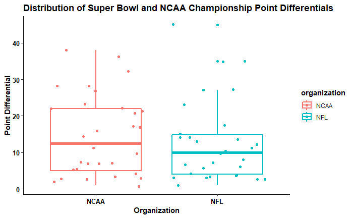
From the above figure, we can see that NFL Super Bowl games have a slightly lower median compared to the NCAA games. It is important to realize that this does not mean that there is statistically significant difference between the two groups. In order to determine if this difference is meaningful we will need to perform some inferential statistics.
We can use permutation testing to see if there is a meaningful difference between the means of the NFL and NCAA point differentials. Briefly, permutation testing allows us to create a null distribution of a statistic of interest (In this case the difference in average point differentials) by shuffling the labels (NCAA and NFL) belonging to the point differentials. We then can generate the mean difference from the resulting shuffle and do this repeatedly.
Permutation Testing: Is there a meaningful difference in the average point differential between the NCAA and NFL championship games?
Calculate observed mean difference in point differential between the NFL and NCAA games
obs_diff <- all_data %>%
  specify(point_differential ~ organization) %>%
  calculate(stat = "diff in means", order = c("NCAA", "NFL"))

#Show observed difference
obs_diff
stat <dbl> | ||||
|---|---|---|---|---|
| 1.866667 |
Create Null distribution
null_distrubution <- all_data %>%
  specify(point_differential ~ organization) %>%
  hypothesize(null = "independence") %>%
  generate(reps = 1000, type = "permute") %>%
  calculate(stat = "diff in means", order = c("NCAA", "NFL"))
Visualize the null distribution and calculate p-value
#visualize null distribution
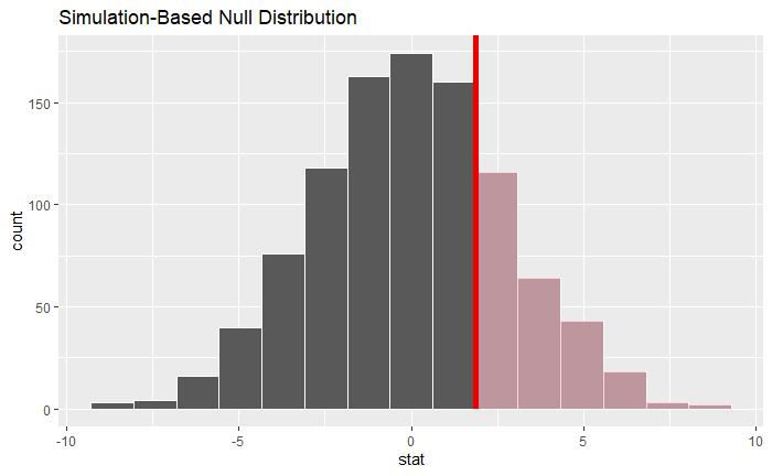
visualise(null_distrubution, bins = 15) +
shade_p_value(obs_stat = obs_diff, direction = "right")
Calculate p-value
#Calculate p-value
null_distrubution %>%
  get_p_value(obs_stat = obs_diff, direction = 'right')
p_value <dbl> | ||||
|---|---|---|---|---|
| 0.246 |
Since the p-value is greater than 0.5, we fail to reject the null hypothesis that the average point differential for Super Bowl games is the same as the average point differential for NCAA championship games. Thus, there is no meaningful difference between the two means.
Is There a Difference In the Proportion of “Blowout” Championship Games Between NCAA and NFL
Though there does not seem to be any agreement on what is a blowout game, it looks like many individuals agree with a number around 17 and 20 plus points.
I am going to make assumption that a 20 point differential is what constitutes a blowout game.
Calculate the number of blowout games
blowouts <- all_data %>%
  mutate(game_status = if_else(point_differential >= 20, true = "blowout", false = "non-blowout")) %>%
  group_by(organization) %>%
  count(game_status)
Visualize data
ggplot(data = blowouts, aes(x = organization, y = n, fill = game_status)) +
  geom_col(color = 'black') +
    ggtitle("Number of Games that were blowout and non-blowout games") +
  ylab("Frequency") +
  xlab("Organization") +
  theme(panel.grid.major = element_blank(),
        panel.grid.minor = element_blank(),
        panel.background = element_blank(),
        axis.line = element_line(colour = 'black'),
        title = element_text(hjust = 0.5, face = 'bold'),
        axis.text.x = element_text(face = 'bold', size = 10, color = 'black'),
        axis.text.y = element_text(face = 'bold', size = 10, color = 'black'),
        axis.title = element_text(color = 'black', face = 'bold'))
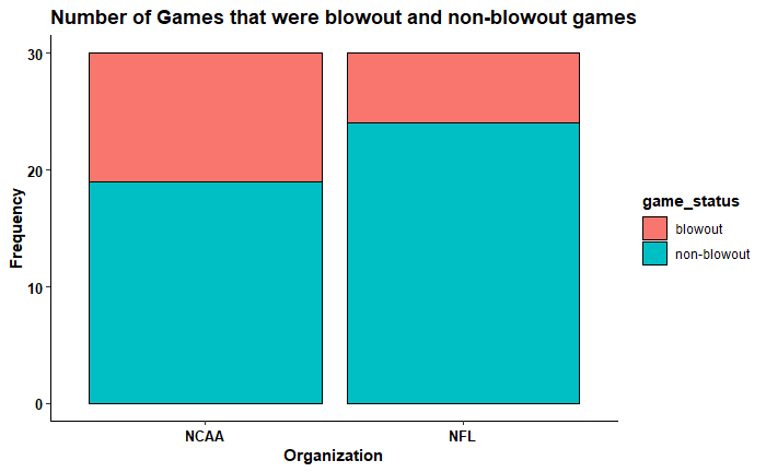
Based on the above figure, there seems to be a larger proportion of NCAA championship games that ended up with a blowout game.
I thought it would be a good idea to calculate the actual percentage of games that were blowouts for both organizations.
Calculate difference in proportion of blowout game between NFL and NCAA Games
blowouts %>%
  group_by(organization) %>%
  mutate(group_total = sum(n)) %>%
  ungroup() %>%
  group_by(organization, game_status) %>%
  summarise(percentage = round((n/group_total)*100, 2)) %>%
  filter(game_status == "blowout")
organization <chr> | game_status <chr> | percentage <dbl> | ||
|---|---|---|---|---|
| NCAA | blowout | 36.67 | ||
| NFL | blowout | 20.00 |
So, we can see that the proportion of games that I considered “blowouts” for the NCAA and NFL championship games was 36.67% and 20% respectively
This means that blowout games occurred 16.67% more in NCAA title games than in Super Bowl games in our sample.
Again, the question is whether or not this is statistically meaningful.
Permutation Testing: Is there a meaningful difference in the proportion of championship blowout games Between NCAA and NFL?
Calculate the observed difference in proportion of championship blowout games between NCAA and NFL
#create new df
blowouts <- all_data %>%
  mutate(game_status = if_else(point_differential >= 20, true = "blowout", false = "non-blowout"))

#Calculate obs difference
obs_diff <- blowouts %>%
  specify(game_status ~ organization, success = "blowout") %>%
  calculate(stat = "diff in props", order = c("NCAA", "NFL"))

#Show observed difference
obs_diff
stat <dbl> | ||||
|---|---|---|---|---|
| 0.1666667 |
Create Null distribution
null_distrubution <- blowouts %>%
  specify(game_status ~ organization, success = "blowout") %>%
  hypothesize(null = "independence") %>%
  generate(reps = 1000, type = "permute") %>%
  calculate(stat = "diff in props", order = c("NCAA", "NFL"))
Visualize the null distribution and calculate p-value
set.seed(1234)
#visualize null distribution
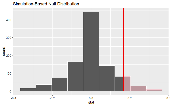
visualise(null_distrubution, bins = 10) +
shade_p_value(obs_stat = obs_diff, direction = "right")
Calculate p-value
#Calculate p-value
null_distrubution %>%
  get_p_value(obs_stat = obs_diff, direction = 'right')
p_value <dbl> | ||||
|---|---|---|---|---|
| 0.121 |