
IMDB Sentiment Classification Project
Data obtained from https://www.kaggle.com/lakshmi25npathi/imdb-dataset-of-50k-movie-reviews
#Import R libraries
library(tidytext) #Sentiment calculation
library(tidyverse) #Data preprocessing
library(quanteda) #Creating document term Matrices
library(reticulate) #Python functions

#Import python libraries
sk_model_selection <- import('sklearn.model_selection') #For test train split
sk.nb <- import('sklearn.naive_bayes') #naive bayes classifier
sk.logistic <- import('sklearn.linear_model') #For logistic regression
sk.metrics <- import('sklearn.metrics') #Accuracy calculation
sk.svm <- import("sklearn.svm") #Support vector machine
sk.ensemble <- import('sklearn.ensemble')  #voting ensemble  classifier
sk.tree <- import('sklearn.tree') #Decision tree  classifier
Data Import and Visualization
# Import data
df <- read_csv('IMDB Dataset.csv')
head(df)
print('Number of Positive and Negtive Reviews')
table(df$sentiment)
| review | sentiment |
|---|---|
| One of the other reviewers has mentioned that after watching just 1 Oz episode you'll be hooked. They are right, as this is exactly what happened with me.<br /><br />The first thing that struck me about Oz was its brutality and unflinching scenes of violence, which set in right from the word GO. Trust me, this is not a show for the faint hearted or timid. This show pulls no punches with regards to drugs, sex or violence. Its is hardcore, in the classic use of the word.<br /><br />It is called OZ as that is the nickname given to the Oswald Maximum Security State Penitentary. It focuses mainly on Emerald City, an experimental section of the prison where all the cells have glass fronts and face inwards, so privacy is not high on the agenda. Em City is home to many..Aryans, Muslims, gangstas, Latinos, Christians, Italians, Irish and more....so scuffles, death stares, dodgy dealings and shady agreements are never far away.<br /><br />I would say the main appeal of the show is due to the fact that it goes where other shows wouldn't dare. Forget pretty pictures painted for mainstream audiences, forget charm, forget romance...OZ doesn't mess around. The first episode I ever saw struck me as so nasty it was surreal, I couldn't say I was ready for it, but as I watched more, I developed a taste for Oz, and got accustomed to the high levels of graphic violence. Not just violence, but injustice (crooked guards who'll be sold out for a nickel, inmates who'll kill on order and get away with it, well mannered, middle class inmates being turned into prison bitches due to their lack of street skills or prison experience) Watching Oz, you may become comfortable with what is uncomfortable viewing....thats if you can get in touch with your darker side. | positive |
| <span style=white-space:pre-wrap>A wonderful little production. <br /><br />The filming technique is very unassuming- very old-time-BBC fashion and gives a comforting, and sometimes discomforting, sense of realism to the entire piece. <br /><br />The actors are extremely well chosen- Michael Sheen not only "has got all the polari" but he has all the voices down pat too! You can truly see the seamless editing guided by the references to Williams' diary entries, not only is it well worth the watching but it is a terrificly written and performed piece. A masterful production about one of the great master's of comedy and his life. <br /><br />The realism really comes home with the little things: the fantasy of the guard which, rather than use the traditional 'dream' techniques remains solid then disappears. It plays on our knowledge and our senses, particularly with the scenes concerning Orton and Halliwell and the sets (particularly of their flat with Halliwell's murals decorating every surface) are terribly well done. </span> | positive |
| <span style=white-space:pre-wrap>I thought this was a wonderful way to spend time on a too hot summer weekend, sitting in the air conditioned theater and watching a light-hearted comedy. The plot is simplistic, but the dialogue is witty and the characters are likable (even the well bread suspected serial killer). While some may be disappointed when they realize this is not Match Point 2: Risk Addiction, I thought it was proof that Woody Allen is still fully in control of the style many of us have grown to love.<br /><br />This was the most I'd laughed at one of Woody's comedies in years (dare I say a decade?). While I've never been impressed with Scarlet Johanson, in this she managed to tone down her "sexy" image and jumped right into a average, but spirited young woman.<br /><br />This may not be the crown jewel of his career, but it was wittier than "Devil Wears Prada" and more interesting than "Superman" a great comedy to go see with friends. </span> | positive |
| <span style=white-space:pre-wrap>Basically there's a family where a little boy (Jake) thinks there's a zombie in his closet & his parents are fighting all the time.<br /><br />This movie is slower than a soap opera... and suddenly, Jake decides to become Rambo and kill the zombie.<br /><br />OK, first of all when you're going to make a film you must Decide if its a thriller or a drama! As a drama the movie is watchable. Parents are divorcing & arguing like in real life. And then we have Jake with his closet which totally ruins all the film! I expected to see a BOOGEYMAN similar movie, and instead i watched a drama with some meaningless thriller spots.<br /><br />3 out of 10 just for the well playing parents & descent dialogs. As for the shots with Jake: just ignore them. </span> | negative |
| <span style=white-space:pre-wrap>Petter Mattei's "Love in the Time of Money" is a visually stunning film to watch. Mr. Mattei offers us a vivid portrait about human relations. This is a movie that seems to be telling us what money, power and success do to people in the different situations we encounter. <br /><br />This being a variation on the Arthur Schnitzler's play about the same theme, the director transfers the action to the present time New York where all these different characters meet and connect. Each one is connected in one way, or another to the next person, but no one seems to know the previous point of contact. Stylishly, the film has a sophisticated luxurious look. We are taken to see how these people live and the world they live in their own habitat.<br /><br />The only thing one gets out of all these souls in the picture is the different stages of loneliness each one inhabits. A big city is not exactly the best place in which human relations find sincere fulfillment, as one discerns is the case with most of the people we encounter.<br /><br />The acting is good under Mr. Mattei's direction. Steve Buscemi, Rosario Dawson, Carol Kane, Michael Imperioli, Adrian Grenier, and the rest of the talented cast, make these characters come alive.<br /><br />We wish Mr. Mattei good luck and await anxiously for his next work. </span> | positive |
| Probably my all-time favorite movie, a story of selflessness, sacrifice and dedication to a noble cause, but it's not preachy or boring. It just never gets old, despite my having seen it some 15 or more times in the last 25 years. Paul Lukas' performance brings tears to my eyes, and Bette Davis, in one of her very few truly sympathetic roles, is a delight. The kids are, as grandma says, more like "dressed-up midgets" than children, but that only makes them more fun to watch. And the mother's slow awakening to what's happening in the world and under her own roof is believable and startling. If I had a dozen thumbs, they'd all be "up" for this movie. | positive |
[1] "Number of Positive and Negtive Reviews"
negative positive
   25000    25000
Calculate difference in sentiment to assess how well reviews match sentiment scores
df$id <- 1:number_reviews #Assign ids to each review
####################### Calculate positive and negative sentiment  (using tidytext) #######################
colnames(df)[2] <- 'Rating' #Change sentiment column name so that tidytext recognizes sentiment column
df_tidy <- df %>%
  group_by(id) %>% #Group by id (id = review)
  unnest_tokens(word, review) %>% #Tokenize words
  anti_join(stop_words, by = 'word') %>% #Remove stop words
  inner_join(get_sentiments('bing'), by = 'word') %>% #Find positive and negative words
  count(sentiment) %>% #Count positive and negative words
  spread(sentiment, n, fill = 0) %>% #Spread positive and negative sentiment values and fill nas with zeros
  mutate(diff = positive - negative) #Create new column with sentiment difference

df_tidy$Rating <- df$Rating[intersect(df_tidy$id, df$id)] #Find reviews that were not removed from join operations


#Plot Difference in Sentiment (Collapsed by group)
ggplot(data = df_tidy, aes(x = Rating, y = diff, color = Rating)) +
  geom_violin() +
  geom_point(alpha = .2) +
  geom_hline(yintercept = 0, linetype = 'dashed') +
  ylab('Difference in Sentiment (Positive - Negative)') +
  xlab('Review Rating') +
  ggtitle('Difference in Sentiment') +
  theme(plot.title = element_text(hjust = 0.5))
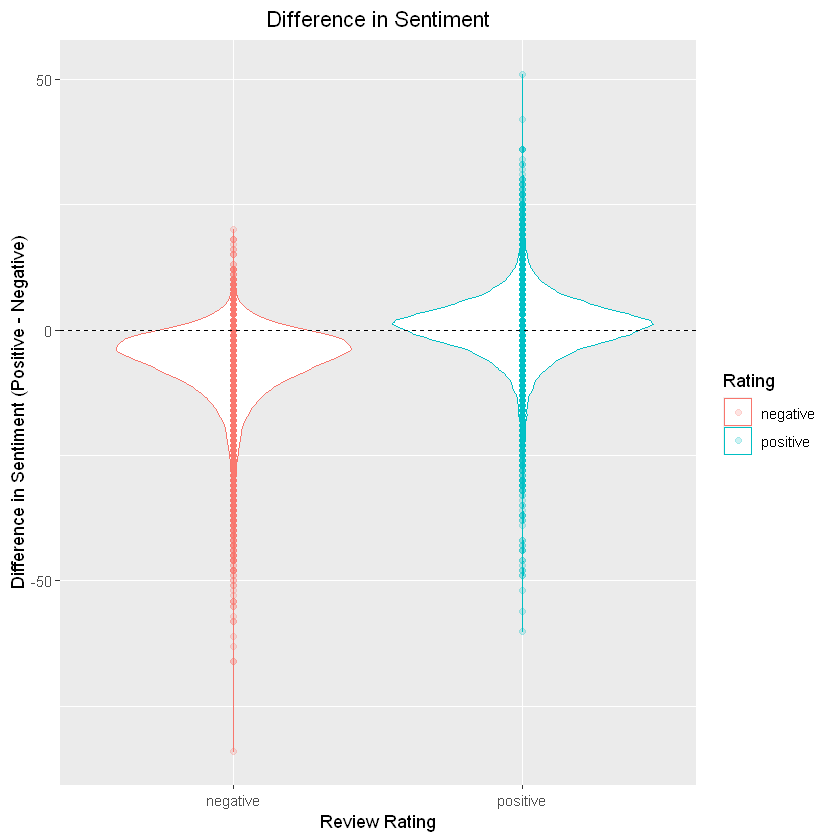
Based on the above violin plots, the positive reviews do seem to tend toward being more positive than the negative reviews
Data Cleaning Step (unigrams only)
##################### Data Preprocessing ######################
df2 <- df #To not overwrite original data frame
number_reviews <- nrow(df2) #Calculate the number of reviews
for(current_review in 1:number_reviews){
  #Remove numbers, punctuation, and symbols
  cleaned_review <- tokens(df2$review[current_review], remove_numbers = T,
                           remove_punct  = T,  remove_symbols = T,
                           remove_separators = T)
  tok_ngrams <- tokens_ngrams(cleaned_review, n = 1) #Extract unigrams

#Store in data frame (Here, I concatenate the strings for the quanteda functions)
  df2$review[current_review] <- paste(unlist(tok_ngrams[["text1"]]), collapse = " ")
}

#Create a document term-frequency matrix and remove stop words
dv <- df2$Rating #For training and testing data
df2 <-df2[, c('review', 'id')] #Rename columns
corpus <- corpus(df2, text_field = 'review', doc_field = 'id') #Create corpus object
dfm <-  dfm(corpus, tolower = T, remove = stopwords('english')) #Calculate document term-frequency matrix
Model training and evaluation (I will be using Sklearn’s functions in this section)
Split data into training and testing sets
####################### perform train test split #######################
#Create test train split
split <- sk_model_selection$train_test_split(dfm, dv, test_size = 0.3, stratify = dv,
                                             random_state = as.integer(7))

X_train <- split[[1]] #Extract training set (Features)
X_test <- split[[2]] #Extract testing set (Features)
y_train <- split[[3]] #Extract training set (target)
y_test <- split[[4]] #Extract testing set (target)
Logistic regression
#### Logistic Regression ####
log_estimator <- sk.logistic$LogisticRegression(max_iter = 1000) #Model parameters
log_estimator$fit(X_train, y_train) #Train model
y_pred <- log_estimator$predict(X_test) #Predict testing data
logistic_accuracy <- sk.metrics$accuracy_score(y_test, y_pred) #accuracy
print(paste('Logistic Accuracy = ', logistic_accuracy))
LogisticRegression(max_iter=1000.0)
[1] "Logistic Accuracy =  0.884266666666667"
Naive Bayes
### Naive Bayes ###
nb_estimator <- sk.nb$MultinomialNB() #Initialize model
nb_estimator$fit(X_train, y_train) #Train model
y_pred <- nb_estimator$predict(X_test) #Predict testing data
nb_baseline <- sk.metrics$accuracy_score(y_test, y_pred) #accuracy
print(paste('nb_baseline = ', nb_baseline))
MultinomialNB()
[1] "nb_baseline =  0.863"
Hyperparameter tuning
min_alpha <- 0 #Minimum alpha
max_alpha <- 1#Max alpha
incriment <- 0.001 #Increment step
param_grid <- r_to_py(list(alpha = seq(from = min_alpha, to = max_alpha, by = incriment)))
nb <- sk.nb$MultinomialNB() #Initialize model
#Random grid search of alpha parameter
random_grid_search <- sk_model_selection$RandomizedSearchCV(estimator = nb,
                                                            param_distributions = param_grid,
                                                            n_iter = 60,
                                                            scoring = 'accuracy',
                                                            return_train_score = TRUE,
                                                            cv = as.integer(10),
                                                            random_state = as.integer(7))
estimator <- random_grid_search$fit(X_train, y_train) #Train model
nb_best <- estimator$best_estimator_ #Store best model
y_pred <- nb_best$predict(X_test) #Predict testing data
nb_hp_best <- sk.metrics$accuracy_score(y_test, y_pred) #accuracy
print(paste('nb_hp_best = ', nb_hp_best))
[1] "nb_hp_best = 0.863066666666667"
Linear support vector machine
#### Support vector machine ###
Lsvm_estimator <- sk.svm$LinearSVC(max_iter = 5000) #Model parameters
Lsvm_estimator$fit(X_train, y_train) #Train model
y_pred <- Lsvm_estimator$predict(X_test) #Predict testing data
Lsvm <- sk.metrics$accuracy_score(y_test, y_pred) #accuracy
print(paste('Lsvm = ', Lsvm))
[1] "Lsvm = 0.868466666666667"
Voting Classifier
######## Voting Classifier ##########
#Combine classifiers into list of tuples
estimators <- list(tuple('log_reg', log_estimator), tuple('nb', nb_best),
                   tuple('LSVM', Lsvm_estimator))
ensemble <- sk.ensemble$VotingClassifier(estimators, voting = 'hard') #Majority rules
ensemble$fit(X_train, y_train) #Train Model
y_pred <- ensemble$predict(X_test) #Predict testing data
voting_ensemble <- sk.metrics$accuracy_score(y_test, y_pred)
print(paste('voting_ensemble = ', voting_ensemble))
VotingClassifier(estimators=[('log_reg', LogisticRegression(max_iter=1000.0)),
                             ('nb', MultinomialNB(alpha=0.716)),
                             ('LSVM', LinearSVC(max_iter=5000.0))])


[1] "voting_ensemble =  0.884466666666667"
Graph Results
# Combine results into data frame for ggplot
#Store classifier names
Classifier <- c('logistic_accuracy', 'nb_baseline', 'nb_hp_best',
                'Lsvm', 'voting_ensemble')

#Store classifier results
Accuracy <- c(logistic_accuracy, nb_baseline, nb_hp_best,
             Lsvm, voting_ensemble)
Accuracy <- round(Accuracy, digits = 5)

#Create data frame
results <- as.data.frame(
cbind(Classifier, Accuracy)
)


################## Plot data ##################
ggplot(data = results, aes(x = Classifier, y = Accuracy)) +
    geom_bar(stat = 'identity', color = 'blue', fill = "white") +
    geom_text(aes(label=Accuracy), position=position_dodge(width=0.9), vjust=-0.25) +
    ggtitle("Classifier Results") +
    theme(plot.title = element_text(hjust = 0.5))
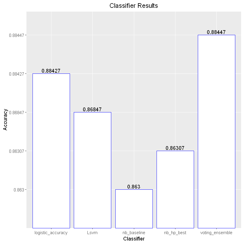
Though the above model accuracies are adequate, they could be much better
Data Cleaning Step (This time with bigrams and trigrams)
##################### Data Preprocessing ######################
df2 <- df #To not overwrite original data frame
number_reviews <- nrow(df2) #Calculate the number of reviews
for(current_review in 1:number_reviews){
  #Remove numbers, punctuation, and symbols
  cleaned_review <- tokens(df2$review[current_review], remove_numbers = T,
                           remove_punct  = T,  remove_symbols = T,
                           remove_separators = T)
  tok_ngrams <- tokens_ngrams(cleaned_review, n = 1:3) #Extract ngrams

#Store in data frame (Here, I concatenate the strings for the quanteda functions)
  df2$review[current_review] <- paste(unlist(tok_ngrams[["text1"]]), collapse = " ")
}

#Create a document term-frequency matrix and remove stop words
dv <- df2$Rating #For training and testing data
df2 <-df2[, c('review', 'id')] #Rename columns
corpus <- corpus(df2, text_field = 'review', doc_field = 'id') #Create corpus object
dfm <-  dfm(corpus, tolower = T, remove = stopwords('english')) #Calculate document term-frequency matrix
Warning message:
"doc_field argument is not used."
Model training and evaluation
Split data into training and testing sets
####################### perform train test split #######################
#Create test train split
split <- sk_model_selection$train_test_split(dfm, dv, test_size = 0.3, stratify = dv,
                                             random_state = as.integer(7))

X_train <- split[[1]] #Extract training set (Features)
X_test <- split[[2]] #Extract testing set (Features)
y_train <- split[[3]] #Extract training set (target)
y_test <- split[[4]] #Extract testing set (target)
Logistic regression
#### Logistic Regression ####
log_estimator <- sk.logistic$LogisticRegression(max_iter = 1000) #Model parameters
log_estimator$fit(X_train, y_train) #Train model
y_pred <- log_estimator$predict(X_test) #Predict testing data
logistic_accuracy <- sk.metrics$accuracy_score(y_test, y_pred) #accuracy
print(paste('Logistic Accuracy = ', logistic_accuracy))
[1] "Logistic Accuracy = 0.9098"
Naive Bayes
### Naive Bayes ###
nb_estimator <- sk.nb$MultinomialNB() #Initialize model
nb_estimator$fit(X_train, y_train) #Train model
y_pred <- nb_estimator$predict(X_test) #Predict testing data
nb_baseline <- sk.metrics$accuracy_score(y_test, y_pred) #accuracy
print(paste('nb_baseline = ', nb_baseline))
[1] "nb_baseline = 0.8998"
Hyperparameter tuning
min_alpha <- 0 #Minimum alpha
max_alpha <- 1#Max alpha
incriment <- 0.001 #Increment step
param_grid <- r_to_py(list(alpha = seq(from = min_alpha, to = max_alpha, by = incriment)))
nb <- sk.nb$MultinomialNB() #Initialize model
#Random grid search of alpha parameter
random_grid_search <- sk_model_selection$RandomizedSearchCV(estimator = nb,
                                                            param_distributions = param_grid,
                                                            n_iter = 60,
                                                            scoring = 'accuracy',
                                                            return_train_score = TRUE,
                                                            cv = as.integer(10),
                                                            random_state = as.integer(7))
estimator <- random_grid_search$fit(X_train, y_train) #Train model
nb_best <- estimator$best_estimator_ #Store best model
y_pred <- nb_best$predict(X_test) #Predict testing data
nb_hp_best <- sk.metrics$accuracy_score(y_test, y_pred) #accuracy
print(paste('nb_hp_best = ', nb_hp_best))
[1] "nb_hp_best = 0.9002"
Linear support vector machine
#### Support vector machine ###
Lsvm_estimator <- sk.svm$LinearSVC(max_iter = 5000) #Model parameters
Lsvm_estimator$fit(X_train, y_train) #Train model
y_pred <- Lsvm_estimator$predict(X_test) #Predict testing data
Lsvm <- sk.metrics$accuracy_score(y_test, y_pred) #accuracy
print(paste('Lsvm = ', Lsvm))
[1] "Lsvm = 0.909266666666667"
Voting Classifier
######## Voting Classifier ##########
#Combine classifiers into list of tuples
estimators <- list(tuple('log_reg', log_estimator), tuple('nb', nb_best),
                   tuple('LSVM', Lsvm_estimator))
ensemble <- sk.ensemble$VotingClassifier(estimators, voting = 'hard') #Majority rules
ensemble$fit(X_train, y_train) #Train Model
y_pred <- ensemble$predict(X_test) #Predict testing data
voting_ensemble <- sk.metrics$accuracy_score(y_test, y_pred)
print(paste('voting_ensemble = ', voting_ensemble))
[1] "voting_ensemble = 0.911866666666667"
Graph Results
# Combine results into data frame for ggplot
#Store classifier names
Classifier <- c('logistic_accuracy', 'nb_baseline', 'nb_hp_best',
                'Lsvm', 'voting_ensemble')

#Store classifier results
Accuracy <- c(logistic_accuracy, nb_baseline, nb_hp_best,
             Lsvm, voting_ensemble)
Accuracy <- round(Accuracy, digits = 5)

#Create data frame
results <- as.data.frame(
cbind(Classifier, Accuracy)
)


################## Plot data ##################
ggplot(data = results, aes(x = Classifier, y = Accuracy)) +
    geom_bar(stat = 'identity', color = 'blue', fill = "white") +
    geom_text(aes(label=Accuracy), position=position_dodge(width=0.9), vjust=-0.25) +
    ggtitle("Classifier Results") +
    theme(plot.title = element_text(hjust = 0.5))
