Mario Party Superstars: Which die block should you buy from the item store?
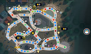
Mario Party Superstars is a Nintendo Switch game where the goal is to travel across virtual game boards to purchase stars. The player with the most stars wins the game. Only one star is out at a time, and varies in distance from players. In most cases, you want to roll as high as possible to ensure you reach the space containing the star before other players. Below is an example of what a board looks like.
To start, each player has a base die block (1 d10) that ranges from 1 to 10. There are other die blocks that you can purchase for one time use: Two 10 sided dice (2 d10s), three 10 sided dice (3 d10s), and a 10 sided die block where you choose what number it lands on (“choose roll”). So my question is, which one should you choose if you can afford them?
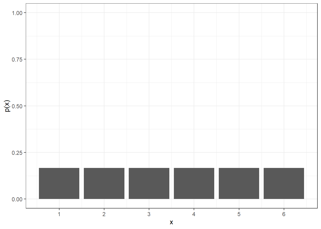
Let’s first consider a standard 6 sided die. How much would we expect to move across the board? Since each number is equally likely, then
or 0.167. So, our random variable (X) follows a discrete uniform distribution.
library(ggplot2)
library(tidyr)
library(dplyr)
library(R6)
x <- 1:6
d <- 1/6
prob_df <- data.frame(x=x, probs = rep(d, 6))

ggplot(prob_df, aes(x=x,y=probs)) +
  geom_bar(stat='identity') +
  ylim(0,1) +
  ylab('p(x)') +
  scale_x_continuous(breaks = x, labels = x) +
  theme_bw()
We can calculate the expected amount of spaces our player will move across the board with a 6 sided die with the following equation: \(E[X] = \sum_{i=1}^{n}p_ix_i\) this weights each value of our die by it’s respective probability. If we expand this out for a 6 sided die we get:
\(E[X] = 1\frac{1}{6} + 2\frac{1}{6} + 3\frac{1}{6} + 4\frac{1}{6}+5\frac{1}{6} + 6\frac{1}{6} = 3.5\)
Now, when we consider our base 10 sided die, the probability of rolling a particular number decreases, but the expected value increases.
x <- 1:10
d <- 1/10
prob_df <- data.frame(x=x, probs = rep(d, 10))

ggplot(prob_df, aes(x=x,y=probs)) +
  geom_bar(stat='identity') +
  ylim(0,1) +
  ylab('p(x)') +
  scale_x_continuous(breaks = x, labels = x) +
  theme_bw()
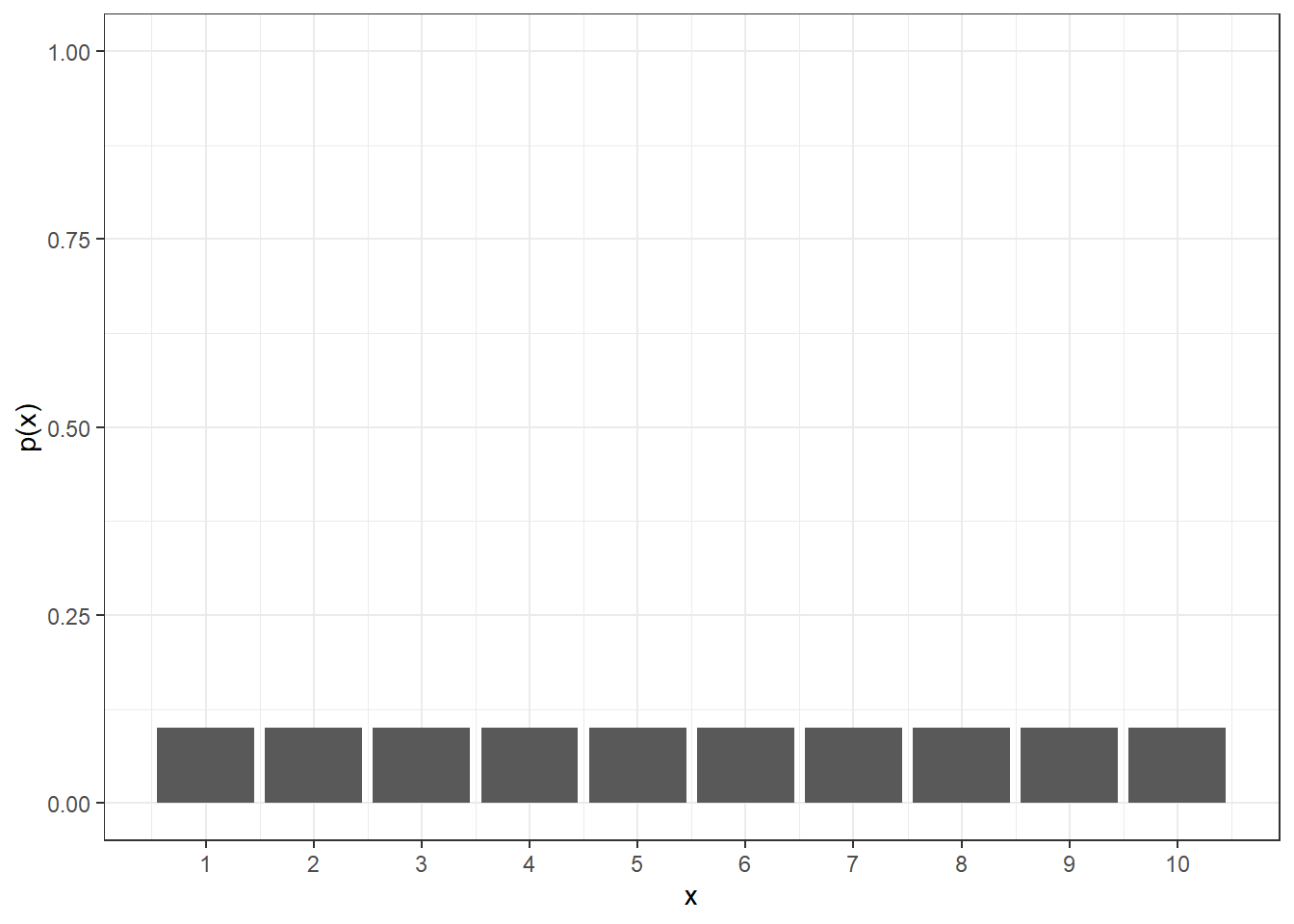
\(E[X] = 1\frac{1}{10} + 2\frac{1}{10} + 3\frac{1}{10} + 4\frac{1}{10} + 5\frac{1}{10} + 6\frac{1}{10} + 7\frac{1}{10} + 8\frac{1}{10} + 9\frac{1}{10} + 10\frac{1}{10}= 5.5\)
Things change when we consider more than 1 die. This is because we sum the values of all dice thrown to know how far we move. Due to the linearity of expectation, we can find out how far a character would move on average (for more than 1 die) by calculating the individual expectations for each die and summing them. More specifically:
Since we know that \(E[X] = 5.5\) for one 10 sided, than \(E[Y]\) for another 10 sided die is the same. \(E[X] = E[Y] = 5.5\)
We can then sum both individual expectations to get: \(E[X] + E[Y] = 11\)
Below is what the probability mass function looks like for summing two 10 sided dice.
d1 <- 1:10
d2 <- 1:10
outcomes <- length(d1) * length(d2)
two_dice <- expand.grid(d1 = d1, d2 = d2) |>
  mutate(sum = d1 + d2) |>
  group_by(sum) |>
  count() |>
  mutate(`p(x)` = n/outcomes)

ggplot(data = two_dice, aes(x=sum,y=`p(x)`)) +
  geom_bar(stat='identity') +
  ylab('p(x)') +
  xlab('die1 + die2') +
  scale_x_continuous(breaks = two_dice$sum, labels = two_dice$sum) +
  theme_bw() +
  theme(panel.grid.major = element_blank(), panel.grid.minor = element_blank())
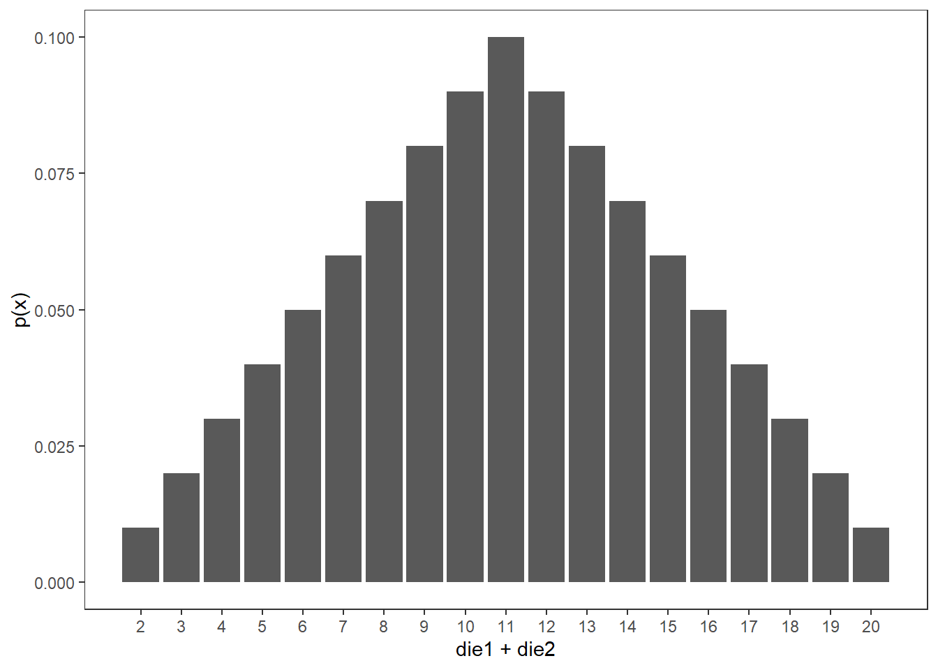
As you can see, the range of possible values is larger for two dice versus one. Not only that, but the probability of rolling at or above the single die maximum (10), is high as well.
#Add grouping
two_dice <- two_dice |>
  mutate(group = if_else(sum >= 10, 'X >= 10', 'X < 10'))

prob_X <- data.frame(prob = sum(two_dice$`p(x)`[two_dice$sum >= 10]))

ggplot() +
  geom_bar(data = two_dice, aes(x=sum, y=`p(x)`, group = group, fill = group), stat='identity') +
  geom_text(data = prob_X, aes(x = 17, y = .099,  group = 1, label = paste('Probability = ', prob*100, '%', sep = '')), color = 'royalblue',  fontface = "bold") +
  ylab('p(x)') +
  xlab('die1 + die2') +
  scale_x_continuous(breaks = two_dice$sum, labels = two_dice$sum) +
  scale_fill_manual(breaks = c('X >= 10', 'X < 10'), values = c(
    'X >= 10' = 'royalblue',
    'X < 10' = NA
  )) +
  theme_bw() +
  theme(panel.grid.major = element_blank(), panel.grid.minor = element_blank()) +
  labs(fill="")
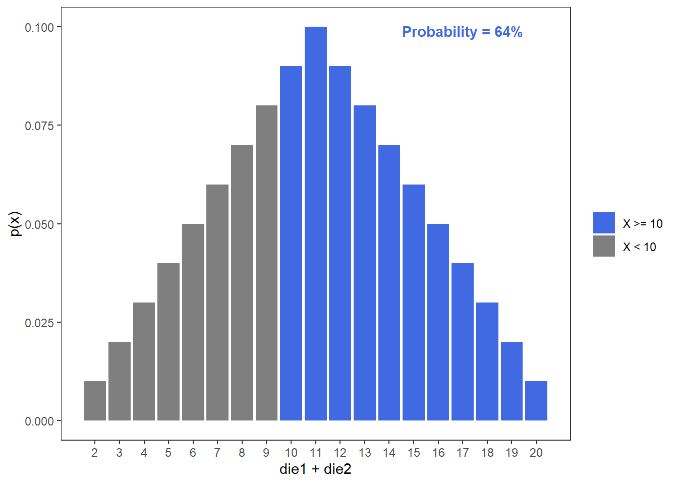
This tells us that we have a 64% chance of rolling at or above a 10 when we have two dice. Much higher than the 10% chance we would have of rolling a 10 with one die.
Therefore, it is no surprise that buying two dice is better than 1, but how does the “choose roll” die block compare? This die block allows you to roll a value between 1 and 10 with absolute certainty. So instead of having a 10% chance of rolling a 10 with the base die, we have a 100% chance of rolling a 10 (or any value for that matter).

This comparison is interesting because there is no variability in the rolls for this die block. This is not true for the base single or pair of dice. You have a better than 50% (p = .64) chance of rolling greater than or equal to a 10 with the two dice. In contrast, you have a 36% (1-p) chance of rolling less than a 10. If we consider the expectation of two 10 sided dice, we know that on average we would expect to move 11 spaces. This is higher than the max value of the “choose roll” die block, though not by much. One way to test which die block moves you further is to simulate it!
What I am going to do is simulate 20 turns (rolls) and calculate the cumulative distance traveled by two players. One player will use the “choose roll” die block exclusively (assume the player will always choose 10) and the other will use two 10 sided dice exclusively.
# Create dice
d1 <- 1:10
d2 <- 1:10

# Number of turns in game
turns <- 20

# Initalize player 1 with 0 movement
player1 <- rep(0, turns)

# Initialize player 2 with all 10s since they have the choose you're own
player2 <- rep(10, turns)

set.seed(123)
for(current_turn in 1:turns){
  # Roll for player 1
  player1[current_turn] <- sample(d1, 1) + sample(d2, 1)
}

#Calculate cumulative movement
player1_cumu <- cumsum(player1)
player2_cumu <- cumsum(player2)

#Create df for ggplot
movement  <- data.frame(turns = c(1:turns, 1:turns),
                        player = c(rep('player 1 (2 dice)', turns), rep('player 2 (choose roll)', turns)),
                        cumulative_movement = c(player1_cumu, player2_cumu)
)

ggplot(data = movement, aes(x = turns, y = cumulative_movement, group = player, color = player)) +
  geom_line(lwd = .8) +
  scale_color_manual(values = c('royalblue', 'gray')) +
  theme_bw() +
  ylab('Cumulative Movement') +
  xlab('Turn') +
  ylim(0, 400) +
  ggtitle('Distance Travaled By Simulated Player')
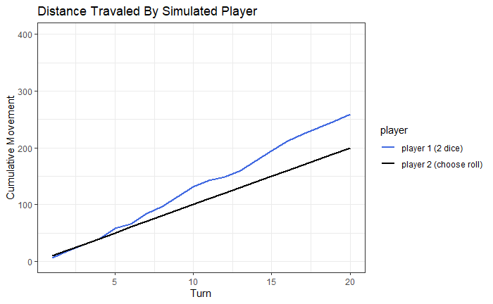
It looks like player 1 with the two 10 sided dice traveled the furthest for this particular game. It is important to note that this only represents one game and the outcome might be different if we play multiple games. Let’s simulate 100 games and see what happens.
set.seed(123)

# Create dice
d1 <- 1:10
d2 <- 1:10

# Number of turns in game
turns <- 20

# Number of games
games <- 100

#initialize list for game results
game_results <- list()

#Simulate games
for(current_game in 1:games){
  # Initalize player 1 with 0 movement
  player1 <- rep(0, turns)

  for(current_turn in 1:turns){
    # Roll for player 1
    player1[current_turn] <- sample(d1, 1) + sample(d2, 1)
  }

  #Calculate cumulative movement
  player1_cumu <- cumsum(player1)

  #Create df for ggplot
  game_results[[current_game]]  <- data.frame(
                          game = rep(current_game, turns),
                          turns = 1:turns,
                          player = rep('player 1 (2 dice)', turns),
                          cumulative_movement = player1_cumu)
}


#Combine games into data frame
all_games_player1 <- bind_rows(game_results)
all_games_player2 <- data.frame(
                          turns = 1:turns,
                          player = rep('player 2 (choose roll)', turns),
                          cumulative_movement = cumsum(rep(10, turns)))


#plot data
ggplot() +
  geom_line(data = all_games_player1, aes(x = turns, y = cumulative_movement, group = game, color = 'player 1 (2 dice)'), lwd = .8, alpha = .2) +
  geom_line(data = all_games_player2, aes(x = turns, y = cumulative_movement, group = 1, color = 'player 2 (choose roll)'), lwd = .8) +
  scale_color_manual(name = 'player',values = c(
  'player 1 (2 dice)' = 'royalblue',
  'player 2 (choose roll)' = 'black')
  ) +
  theme_bw() +
  ylab('Cumulative Movement') +
  xlab('Turn') +
  ylim(0, 400) +
  ggtitle('Distance Travaled By Simulated Player')
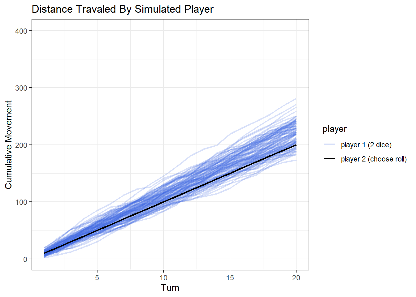
We can see that player 2 now has some games with a higher cumulative distance than player 1. Though it looks like player 1 moved further for the majority of the games. We can actually quantify who moved further across all games.
# Get the max value for each game for player 1
player1_ending_value <- all_games_player1 %>%
  group_by(game) %>%
  summarise(total_moves = max(cumulative_movement))

#Get max value for player 2
player2_ending_value <- max(all_games_player2$cumulative_movement)

# calculate wins by player
wins_by_distance_traveled <- player1_ending_value %>%
  mutate(most_moved_player = case_when(
    total_moves > player2_ending_value ~ 'player 1',
    total_moves < player2_ending_value ~ 'player 2',
    total_moves == player2_ending_value ~ 'tie'
  )) %>%
  group_by(most_moved_player) %>%
  count()


#plot data
ggplot(data = wins_by_distance_traveled, aes(x = most_moved_player, y = n)) +
  geom_bar(stat = 'identity') +
  theme_bw() +
  geom_text(aes(label = n), nudge_y = 2) +
  ylab('Wins (in terms of distance traveled)') +
  xlab('player')
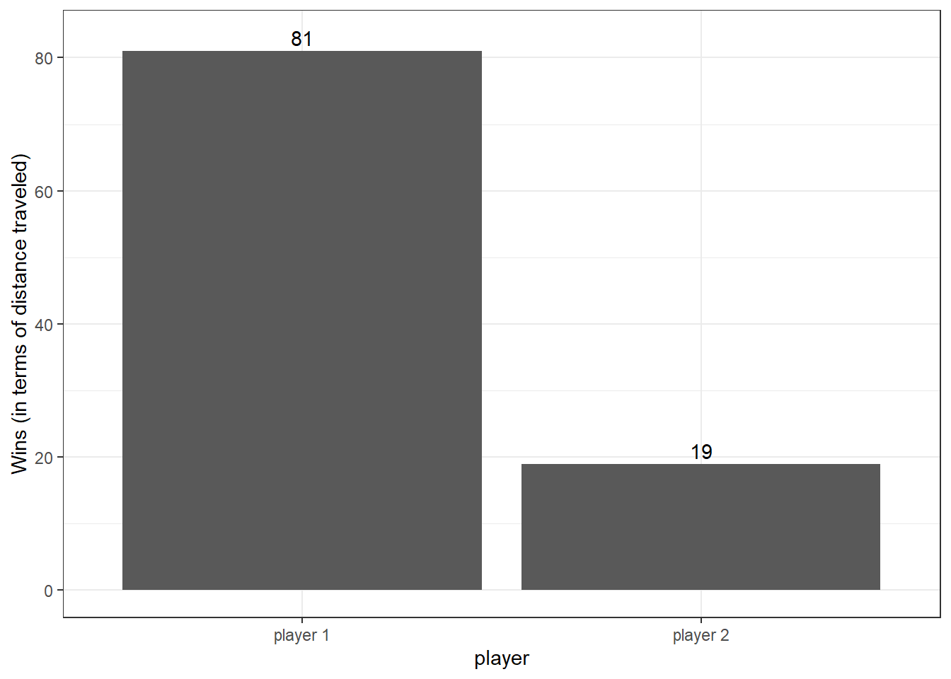
Out of the 100 games, player 1 (two dice) had the highest cumulative distance for 81 games compared to player 2 (“choose roll” die block) who had the highest cumulative distance for 19 games.
One thing that I think is neat is that we can confirm our expectation calculation for the two 10 sided dice by fitting a linear regression model on all the simulated games for player 1.
model <- lm(data = all_games_player1, cumulative_movement ~ turns)
summary(model)
Call:
lm(formula = cumulative_movement ~ turns, data = all_games_player1)

Residuals:
    Min      1Q  Median      3Q     Max
-47.362  -8.896  -0.667   8.186  60.638

Coefficients:
            Estimate Std. Error t value Pr(>|t|)
(Intercept) -0.36911    0.65378  -0.565    0.572
turns       11.03653    0.05458 202.220   <2e-16 ***
---
Signif. codes:  0 '***' 0.001 '**' 0.01 '*' 0.05 '.' 0.1 ' ' 1

Residual standard error: 14.07 on 1998 degrees of freedom
Multiple R-squared:  0.9534,    Adjusted R-squared:  0.9534
F-statistic: 4.089e+04 on 1 and 1998 DF,  p-value: < 2.2e-16
The above output tells us that on average we should expect our player’s cumulative distance to increase by 11.04 (coefficient for turns) for each turn that goes by. Very close to our calculation above that gave us an expected value of 11.
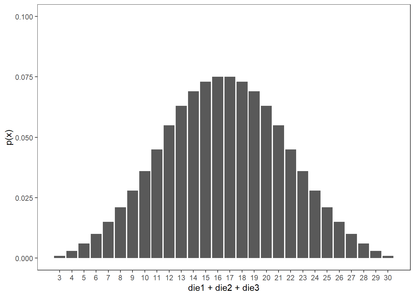
Now let’s take a look at what would happen if we buy three 10 sided dice (3 d10s). Following what we have done in the two dice example, we can just add the expectation of a third die block. That is \(E[X + Y + Z] = 5.5 + 5.5 + 5.5 = 16.5\)
The probability mass function for three 10 sided dice can be seen below.
d1 <- 1:10
d2 <- 1:10
d3 <- 1:10
outcomes <- length(d1) * length(d2) * length(d3)
three_dice <- expand.grid(d1 = d1, d2 = d2, d3 = d3) |>
  mutate(sum = d1 + d2 + d3) |>
  group_by(sum) |>
  count() |>
  mutate(`p(x)` = n/outcomes)

ggplot(data = three_dice, aes(x=sum,y=`p(x)`)) +
  geom_bar(stat='identity') +
  ylab('p(x)') +
  xlab('die1 + die2 + die3') +
  scale_x_continuous(breaks = three_dice$sum, labels = three_dice$sum) +
  theme_bw()+
  ylim(0, .1) +
  theme(panel.grid.major = element_blank(), panel.grid.minor = element_blank())
Similar to above, let’s see what the probability of rolling at or above a 20 is for both a pair of dice and three dice.
#Add grouping
three_dice <- three_dice |>
  mutate(group = if_else(sum >= 20, 'X >= 20', 'X < 20'))

prob_X <- data.frame(prob = sum(three_dice$`p(x)`[three_dice$sum >= 20]))

ggplot() +
  geom_bar(data = three_dice, aes(x=sum, y=`p(x)`, group = group, fill = group), stat='identity') +
  geom_text(data = prob_X, aes(x = 25, y = .099,  group = 1, label = paste('Probability = ', prob*100, '%', sep = '')), color = 'royalblue',  fontface = "bold") +
  ylab('p(x)') +
  xlab('die1 + die2') +
  scale_x_continuous(breaks = three_dice$sum, labels = three_dice$sum) +
  scale_fill_manual(breaks = c('X >= 20', 'X < 20'), values = c(
    'X >= 20' = 'royalblue',
    'X < 20' = NA
  )) +
  theme_bw() +
  ylim(0, .1) +
  theme(panel.grid.major = element_blank(), panel.grid.minor = element_blank()) +
  labs(fill="")
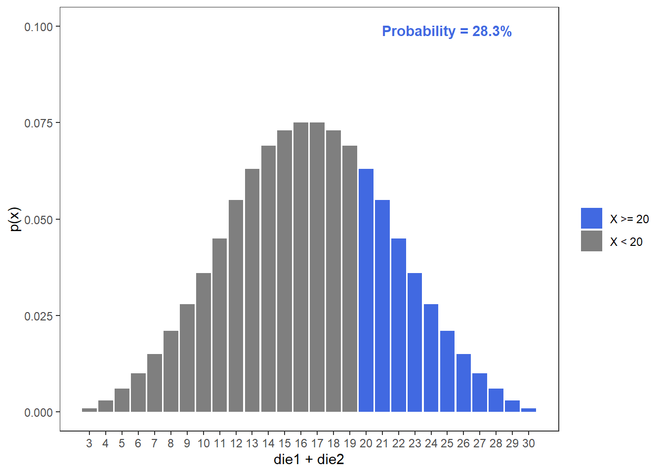
Based on the above figure, the probability of rolling at or above the two dice maximum (20) is 28.3%.
Now let’s run another simulation, this time adding a player who exclusively has three 10 sided dice.
set.seed(123)

# Create dice
d1 <- 1:10
d2 <- 1:10
d3 <-  1:10

# Number of turns in game
turns <- 20

# Number of games
games <- 100

#initialize list for game results
game_results <- list()

#Simulate games
for(current_game in 1:games){
  # Initalize player 1 with 0 movement
  player1 <- rep(0, turns)

  # Initalize player 3 with 0 movement
  player3 <- rep(0, turns)

  for(current_turn in 1:turns){
    # Roll for player 1
    player1[current_turn] <- sample(d1, 1) + sample(d2, 1)
    #Roll for player 3
    player3[current_turn] <- sample(d1, 1) + sample(d2, 1) + sample(d3, 1)

  }

  #Calculate cumulative movement
  player1_cumu <- cumsum(player1)
  player3_cumu <- cumsum(player3)

  #Create df for ggplot
  game_results[[current_game]]  <- data.frame(
                          game = c(rep(current_game, turns), rep(current_game, turns)),
                          turns = c(1:turns, 1:turns),
                          player = c(rep('player 1 (2 dice)', turns), rep('player 3 (3 dice)', turns)),
                          cumulative_movement = c(player1_cumu, player3_cumu))
}


#Combine games into data frame
all_games_player13 <- bind_rows(game_results)
all_games_player2 <- data.frame(
                          turns = 1:turns,
                          player = rep('player 2 (choose roll)', turns),
                          cumulative_movement = cumsum(rep(10, turns)))

#plot data
ggplot() +
  geom_boxplot(data = all_games_player13, aes(x = as.factor(turns), y = cumulative_movement, color = player))  +
  geom_point(data = all_games_player2, aes(x = turns, y = cumulative_movement, color = 'player 2 (choose roll)')) +
  theme_bw() +
  scale_color_manual(name = 'player',values = c(
  'player 1 (2 dice)' = 'royalblue',
  'player 2 (choose roll)' = 'black',
  'player 3 (3 dice)' = 'darkgreen')
  ) +
  ylab('Cumulative Movement') +
  xlab('Turn') +
  ylim(0, 400) +
  ggtitle('Distance Travaled By Simulated Player')
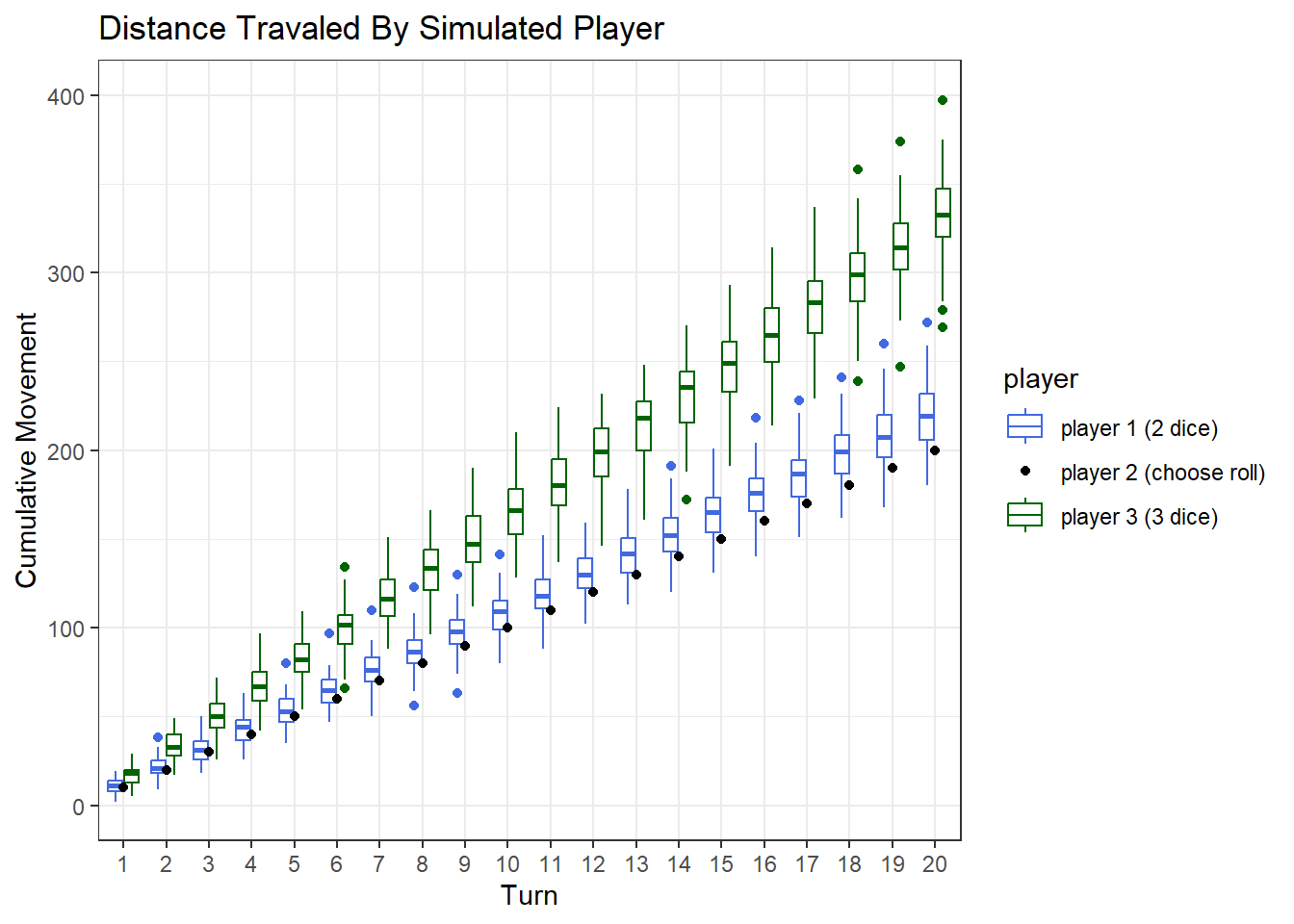
If we look at turn 20 alone, it seems clear that player 3 crushes the competition. Player 2’s boxplot does not overlap with player 3’s box-plot at all with the exception of one outlier game.
#Get max value for player 2
player2_ending_value <- max(all_games_player2$cumulative_movement)

# Get the max value for each game for player 1 and 3
all_game_outcomes <- all_games_player13 %>%
  group_by(game, player) %>%
  summarise(total_moves = max(cumulative_movement)) %>%
  ungroup() %>%
  pivot_wider(id_cols = game,names_from = player, values_from = total_moves) %>%
  mutate(`player 2 (choose roll)` = player2_ending_value,
         most_moved_player = case_when(
          `player 1 (2 dice)` >  `player 2 (choose roll)`  &
          `player 1 (2 dice)` >  `player 3 (3 dice)` ~  'player 1 (2 dice)',

          `player 2 (choose roll)` >  `player 1 (2 dice)`  &
          `player 2 (choose roll)`>  `player 3 (3 dice)` ~ "player 2 (choose roll)",

          `player 3 (3 dice)` >  `player 2 (choose roll)`  &
          `player 3 (3 dice)` >  `player 1 (2 dice)` ~  'player 3 (3 dice)'
         )) %>%
  group_by(most_moved_player) %>%
  count()


#plot data
ggplot(data = all_game_outcomes, aes(x = most_moved_player, y = n)) +
  geom_bar(stat = 'identity') +
  theme_bw() +
  geom_text(aes(label = n), nudge_y = 2) +
  ylab('Wins (in terms of distance traveled)') +
  xlab('player')
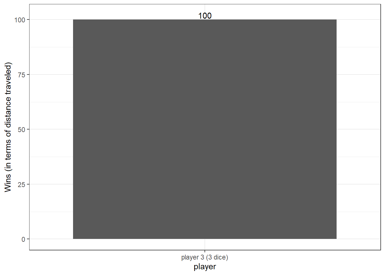
In terms of distance traveled, player 3 moved the most in all 100 games.
The last thing I would like to simulate here is an actual game board where stars will be placed randomly across the board. If a player lands at a space with a star, we will assume the player will purchase said star. Once a purchase occurs, the star will be randomly placed on the board again.
set.seed(123)

x <- c(rep(0, 20), 0:19, rep(19, 20), 19:0)
y <-  c(0:19, rep(20, 20), 19:0, rep(0, 20))
idx <- 1:length(x)
game_board <- data.frame(
  x = x,
  y = y,
  idx = idx
) %>% mutate(`Star Location` = if_else(idx == sample(idx, 1), 'Star Location', 'Regular Space'))


ggplot(data = game_board, aes(x = x, y = y, group = 1, color = `Star Location`)) +
  geom_point(size = 2) +
  geom_text(aes(x = -1, 0, label = "start"), color = 'royalblue') +
  scale_color_manual(breaks = c('Regular Space', 'Star Location'),
                     values = c('Regular Space' = 'black',
                                'Star Location' = 'red'
                                )) +
   theme(axis.line=element_blank(),axis.text.x=element_blank(),
          axis.text.y=element_blank(),axis.ticks=element_blank(),
          axis.title.x=element_blank(),
          axis.title.y=element_blank(),
          panel.background=element_blank(),panel.border=element_blank(),panel.grid.major=element_blank(),
          panel.grid.minor=element_blank(),plot.background=element_blank()) +
  geom_segment(aes(x = -1, y = 1, xend = -1, yend = 20), arrow = arrow(), lwd = 1, color = 'darkgray') +
  geom_segment(aes(x = -1, y = 21, xend = 19, yend = 21), arrow = arrow(), lwd = 1, color = 'darkgray') +
    geom_segment(aes(x = 20, y = 21, xend = 20, yend = 0), arrow = arrow(), lwd = 1, color = 'darkgray') +
      geom_segment(aes(x = 20, y = -1, xend = 0, yend = -1), arrow = arrow(), lwd = 1, color = 'darkgray') +
  geom_text(aes(x = 10, y = 10, label = "Simulated Mario Party Game Board"), color = 'red',  size = 5, fontface = "bold")
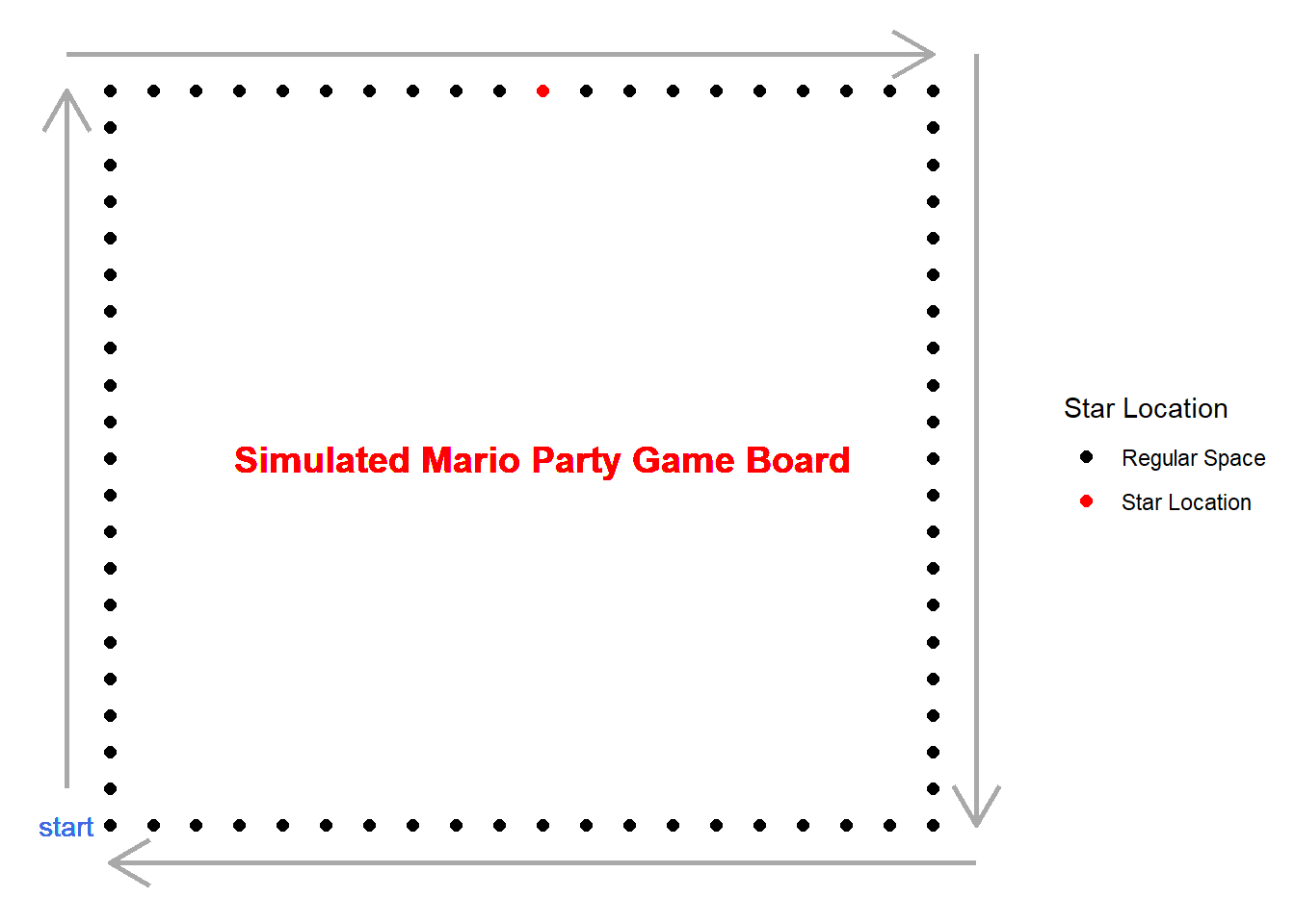
This is defintly not a good looking game, but this will be the board I use for the simulation. Note that each space has an index assigned to it, which will determine where the player is located. You can see that a star has been placed at an index randomly. The first player to get to this space first will get the star.
Let’s create and run the simulation!
The first thing I am going to do is use the R6 library to create a “player” object. The player object will have several attributes: Name, dice type, rolls, and stars.
# Create a player object using R6 that contains die type and position of player
player <- R6Class("player", list(
  name = NULL, #player name
  die = NA, #dice type of player
  position = 1, #starting position
  rolls = c(), #initialize rolls
  stars = 0 #initialize number of stars
Name is arbitrary for the object. Die is initialized as NA but will be important for a method I define in the next section. The position attribute is initialized at 1 so that each player has the same starting point. Rolls is initialized as an empty vector that will store the roll a player had during a given turn. Stars is the number of stars a player has reached.
Next I will define an initialize method. When an object is created, the name and die type are defined by the user.
initialize = function(name, die){
  self$name <- name
  self$die <- die
}
The roll_move method is dictated by the die type the player is assigned. In the above example, the object checks the die type in an “if” statement and uses the rolling capabilities of that die type. When a roll occurs, it is stored in the rolls attribute. Next, I calculate the spaces the player will visit and store those indices in the visted_spaces variable. It is possible that the roll might exceed the game boards maximum index. For those spaces that are above said maximum, I subtract the max index. This way the player keeps going around the board.
roll_move = function(){
    die <- 1:10
    #Calculate movement for 1 d10 (i.e. 1 10 sided die)
    if(self$die == "1 d10"){
      #Roll
      current_roll = sample(die, 1)

      #Append to rolls attribute
      self$rolls <- c(self$rolls, current_roll)

      # figure out rolls that take player pass highest index
      visted_spaces <-  self$position:(self$position + current_roll)

      #Subtract highest index from rolls that go past starting point
      visted_spaces[visted_spaces > max(game_board$idx)] <- visted_spaces[visted_spaces > max(game_board$idx)] - max(game_board$idx)
    }
}
Lastly, I loop through each space the player lands on and check to see if that index contains a star. If there is a star located at that index, I increment the star attribute by 1.
#Initiate player movement
  for(curr_position in visted_spaces){
    #Player must pass star location to get star
    if(curr_position == star_location & self$position != star_location){
      self$stars <- self$stars + 1
    }
  }
  self$position <- tail(visted_spaces, n=1)
The only other method in the object allows for printing useful information on the player.
print = function(...){
  cat("Player name: ", self$name, "\n")
  cat("Die of player: ", self$die , "\n")
  cat("Position of player: ", self$position , "\n")
  cat("Number of stars: ", self$stars , "\n")
}
The full code can be seen below.
# Create a player object using R6 that contains die type and position of player
player <- R6Class("player", list(
  name = NULL, #player name
  die = NA, #dice type of player
  position = 1, #starting position
  rolls = c(), #initialize rolls
  stars = 0, #initialize number of stars
  initialize = function(name, die){
    self$name <- name
    self$die <- die
  },
  roll_move = function(){
    die <- 1:10
    #Calculate movement for 1 d10 (i.e. 1 10 sided die)
    if(self$die == "1 d10"){
      #Roll
      current_roll = sample(die, 1)

      #Append to rolls attribute
      self$rolls <- c(self$rolls, current_roll)

      # figure out rolls that take player pass highest index
      visted_spaces <-  self$position:(self$position + current_roll)

      #Subtract highest index from rolls that go past starting point
      visted_spaces[visted_spaces > max(game_board$idx)] <- visted_spaces[visted_spaces > max(game_board$idx)] - max(game_board$idx)

  #Initiate player movement
  for(curr_position in visted_spaces){
    #Player must pass star location to get star
    if(curr_position == star_location & self$position != star_location){
      self$stars <- self$stars + 1
    }
  }
  self$position <- tail(visted_spaces, n=1)

    }
    # Calculate movement for 2 d10s
    else if(self$die == "2 d10"){
      #Roll
      current_roll = sample(die, 1) + sample(die, 1)

      #Append to rolls attribute
      self$rolls <- c(self$rolls, current_roll)

      #Subtract highest index from rolls that go past starting point
      visted_spaces <-  self$position:(self$position + current_roll)

      #Sub tract highest index
      visted_spaces[visted_spaces > max(game_board$idx)] <- visted_spaces[visted_spaces > max(game_board$idx)] - max(game_board$idx)
  #Initiate player movement
  for(curr_position in visted_spaces){
    #Player must pass star location to get star
    if(curr_position == star_location & self$position != star_location){
      self$stars <- self$stars + 1
    }
  }
  self$position <- tail(visted_spaces, n=1)
    }
    # Calculate movement for 3 d10s
    else if(self$die == "3 d10"){
      #Roll
      current_roll <- sample(die, 1) + sample(die, 1) + sample(die, 1)

      #Append to rolls attribute
      self$rolls <- c(self$rolls, current_roll)

      #Subtract highest index from rolls that go past starting point
      visted_spaces <-  self$position:(self$position + current_roll)

      #Subtract highest index
      visted_spaces[visted_spaces > max(game_board$idx)] <- visted_spaces[visted_spaces > max(game_board$idx)] - max(game_board$idx)

  #Initiate player movement
  for(curr_position in visted_spaces){
    #Player must pass star location to get star
    if(curr_position == star_location & self$position != star_location){
      self$stars <- self$stars + 1
    }
  }
  self$position <- tail(visted_spaces, n=1)
    }
    # Calculate movement for choose roll
    else if(self$die == "choose roll"){
      #Roll (assuming highest value will be picked)
      current_roll <- 10

      #Append to rolls attribute
      self$rolls <- c(self$rolls, current_roll)

      #Subtract highest index from rolls that go past starting point
      visted_spaces <-  self$position:(self$position + current_roll)

      #Subtract highest index
      visted_spaces[visted_spaces > max(game_board$idx)] <- visted_spaces[visted_spaces > max(game_board$idx)] - max(game_board$idx)

  #Initiate player movement
  for(curr_position in visted_spaces){
    #Player must pass star location to get star
    if(curr_position == star_location & self$position != star_location){
      self$stars <- self$stars + 1
    }
  }
  self$position <- tail(visted_spaces, n=1)
    }
  },
  print = function(...){
    cat("Player name: ", self$name, "\n")
    cat("Die of player: ", self$die , "\n")
    cat("Position of player: ", self$position , "\n")
    cat("Number of stars: ", self$stars , "\n")
  }
  )
)
One thing to note is that since I will be randomly placing stars on the board, its possible a star will be placed on the position of a player before they take their turn. The logic I have implemented requires players to take their turn (roll) before they can obtain a star. So if a player ends their turn on position 40, and a star is placed there after they take their turn, they cannot get that star. Players must cross or end at a location with a star to obtain it.
Now let’s simulate our game!
set.seed(123)

#number of turns in game
number_of_turns <- 60

#Initialize players
p1 <- player$new(name = 'Player 1', '1 d10')
p2 <- player$new(name = 'Player 2', '2 d10')
p3 <- player$new(name = 'Player 3', '3 d10')
p4 <- player$new(name = 'Player 4', 'choose roll')

#initialize star location
star_location <- sample(game_board$idx, 1)

#create function that checks if star has been obtained
star_player_check <- function(old_num_stars, new_num_stars, star_location){
  if(new_num_stars > old_num_stars){
    return(sample(game_board$idx, 1))
  }
  else{
    return(star_location)
  }
}

for(curr_turn in 1:number_of_turns){
  #check player1 stars
  old_p1_stars <- p1$stars

  #Roll for player 1
  p1$roll_move()

  #check if p1 obtained star
  new_p1_stars <- p1$stars

  #reset star if obtained
  star_location <- star_player_check(old_p1_stars, new_p1_stars, star_location)

  #check player2 stars
  old_p2_stars <- p2$stars

  #Roll for player 1
  p2$roll_move()

  #check if p1 obtained star
  new_p2_stars <- p2$stars

  #reset star if obtained
  star_location <- star_player_check(old_p2_stars, new_p2_stars, star_location)

  #check player3 stars
  old_p3_stars <- p3$stars

  #Roll for player 1
  p3$roll_move()

  #check if p1 obtained star
  new_p3_stars <- p3$stars

  #reset star if obtained
  star_location <- star_player_check(old_p3_stars, new_p3_stars, star_location)

  #check player4 stars
  old_p4_stars <- p4$stars

  #Roll for player 1
  p4$roll_move()

  #check if p1 obtained star
  new_p4_stars <- p4$stars

  #reset star if obtained
  star_location <- star_player_check(old_p4_stars, new_p4_stars, star_location)

}
The above code iterates through 60 turns. Before a player rolls, the number of stars a player has is looked at before and after their respective roll via the “star_player_check function”. If the player reaches a space with a star, the function will assign a new position index to the star. If not, the function returns the same position of the star.
Let’s see who reached the most stars
game_outcome <- data.frame(
  stars = c(p1$stars, p2$stars, p3$stars, p4$stars),
  player = c(p1$die, p2$die, p3$die, p4$die)
  )

ggplot(data = game_outcome, aes(x=reorder(player,-stars), y = stars)) +
  geom_bar(stat='identity') +
  geom_text(aes(label=stars), nudge_y = 1, fontface = "bold") +
  theme_bw() +
  xlab("Dice Type") +
  ggtitle("Number of stars reached by player")
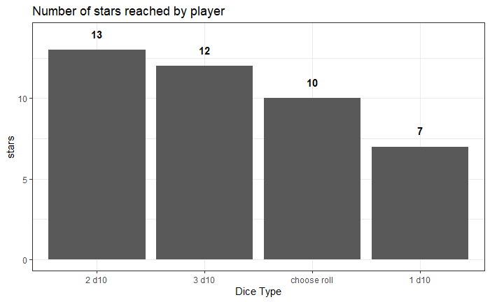
So this is an interesting outcome. Player 2 with 2 d10s reached the most stars. As we have seen above, the player with 3 10s is expected to move the furthest compared to other dice you can buy in the game. It’s possible that for this particular game, player 2 rolled higher than the expected value of 11. Let’s take a look.
game_rolls <- data.frame(
  roll = c(p1$rolls, p2$rolls, p3$rolls, p4$rolls),
  player = c(rep(p1$die, length(p1$rolls)), rep(p2$die, length(p2$rolls)), rep(p3$die, length(p3$rolls)), rep(p4$die, length(p4$rolls)))
  )

ggplot(data = game_rolls, aes(x = player, y = roll)) +
  geom_boxplot(color = 'darkgray') +
  geom_jitter(color = 'royalblue') +
  theme_bw() +
  xlab("Dice Type") +
  ggtitle("Rolls for each player")
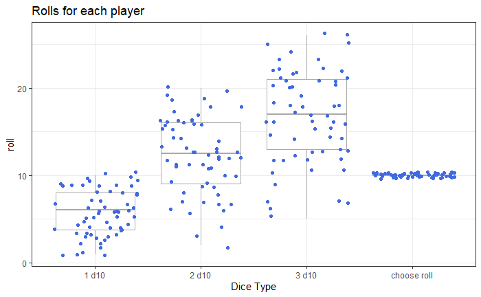
It looks like this is approximatly in line with our expectation calculations. So it is likely that player 2 ended up having stars randomly placed close to them. Let’s now run a simulation with 100 games of 60 turns each.
set.seed(123)
#Number of games to play
number_of_games <- 100

#Number of turns in each game
number_of_turns <- 60

# create list for storing game results
game_results <- list()

#Loop through games
for(current_game in 1:number_of_games){
  #Initialize players
  p1 <- player$new(name = 'Player 1', '1 d10')
  p2 <- player$new(name = 'Player 2', '2 d10')
  p3 <- player$new(name = 'Player 3', '3 d10')
  p4 <- player$new(name = 'Player 4', 'choose roll')

  #initialize star location
  star_location <- sample(game_board$idx, 1)
  #Loop through turns
  for(curr_turn in 1:number_of_turns){
    #check player1 stars
    old_p1_stars <- p1$stars

    #Roll for player 1
    p1$roll_move()

    #check if p1 obtained star
    new_p1_stars <- p1$stars

    #reset star if obtained
    star_location <- star_player_check(old_p1_stars, new_p1_stars, star_location)

    #check player2 stars
    old_p2_stars <- p2$stars

    #Roll for player 1
    p2$roll_move()

    #check if p1 obtained star
    new_p2_stars <- p2$stars

    #reset star if obtained
    star_location <- star_player_check(old_p2_stars, new_p2_stars, star_location)

    #check player3 stars
    old_p3_stars <- p3$stars

    #Roll for player 1
    p3$roll_move()

    #check if p1 obtained star
    new_p3_stars <- p3$stars

    #reset star if obtained
    star_location <- star_player_check(old_p3_stars, new_p3_stars, star_location)

    #check player4 stars
    old_p4_stars <- p4$stars

    #Roll for player 1
    p4$roll_move()

    #check if p1 obtained star
    new_p4_stars <- p4$stars

    #reset star if obtained
    star_location <- star_player_check(old_p4_stars, new_p4_stars, star_location)
  }

  #Create game name
  game_name <- paste('game', current_game, sep = '')


  #Create data frame for game results
  game_outcome <- data.frame(
    stars = c(p1$stars, p2$stars, p3$stars, p4$stars),
    player = c(p1$die, p2$die, p3$die, p4$die),
    game <- rep(game_name, 4)
    )

  #Store data in list
  game_results[[game_name]] <- game_outcome
}
#Combine games
all_games <- bind_rows(game_results)
#Calculate winner of each game
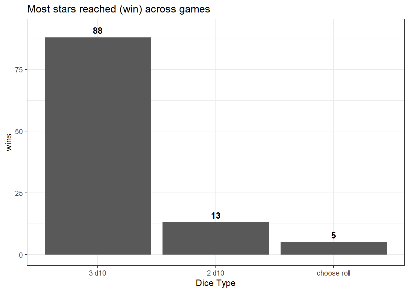
all_games %>%
group_by(game....rep.game_name..4.) %>%
filter(stars == max(stars)) %>%
group_by(player) %>%
summarise(wins = n()) %>%
ggplot(aes(x=reorder(player,-wins), y = wins)) +
geom_bar(stat='identity') +
geom_text(aes(label=wins), nudge_y = 3, fontface = "bold") +
theme_bw() +
xlab("Dice Type") +
ggtitle("Most stars reached (win) across games")
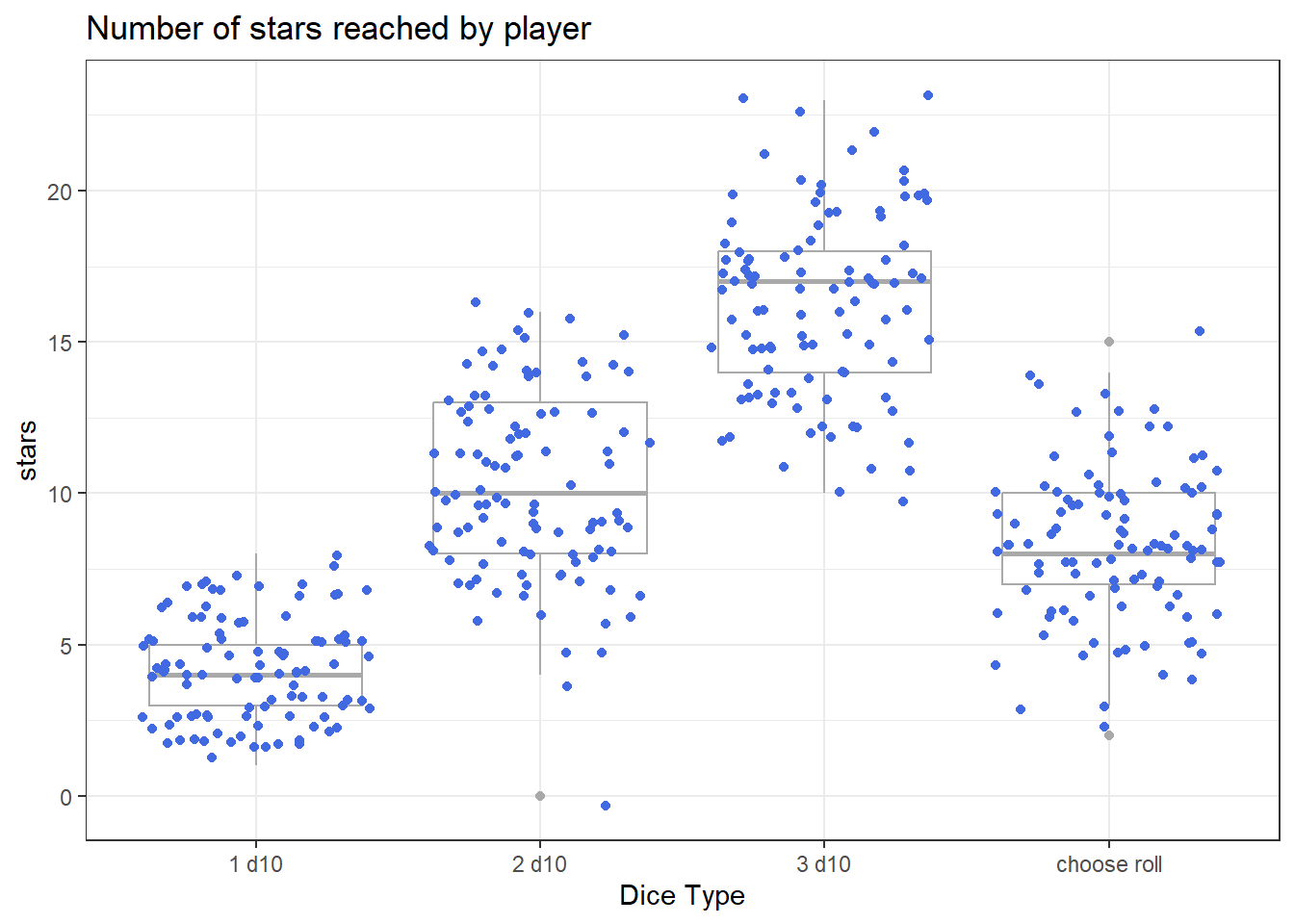
ggplot(data = all_games, aes(x = player, y = stars)) +
  geom_boxplot(color = 'darkgray') +
  geom_jitter(color = 'royalblue') +
  theme_bw() +
  xlab("Dice Type") +
  ggtitle("Number of stars reached by player")