Calculating the Intercept and Regression Coefficient using the Matrix Inverse in Python

In linear regression, we map the predictor variable/s X to the dependent variable Y with the linear function Y = f(x) = a + bx

You can think about this as solving a system of linear equations. For example, if we had an independent and dependent variable with n observations, we could write out the series of equations like this…

We can change the representation of the linear system using matrix notation.

Matrix equation: Ax = b where A is the matrix containing predictors, x is the matrix containing the coefficients, and b is the target/dependent variable.

We can solve for x (a and b) by performing the following operations

\begin{equation}(A^{T}A)^{-1}(A^{T}A)x = (A^{T}A)^{-1}A^{T}b \ or \ x = (A^{T}A)^{-1}A^{T}b\end{equation}

Let’s import some data and use Python to test some of what we discussed

# Import libraries
import pandas as pd 
import numpy as np
import matplotlib.pyplot as plt
from sklearn.linear_model import LinearRegression

# Import synthetic dataset 
data = pd.read_csv("C:\\Users\\steve\\OneDrive\\Documents\\website projects\\statistics\\synthetic data\\simple_regression.csv")
#View dataframe
data.head()

	Unnamed: 0	x	y
0	1	4.373518	89.996377
1	2	4.723557	96.019228
2	3	5.671688	116.386921
3	4	4.860543	100.563548
4	5	4.797259	100.377688

# Visualize data using matplotlib
plt.scatter(data.x, data.y, edgecolor = "black")
plt.xlabel("x - Independent Variable")
plt.ylabel("y - Dependent Variable")

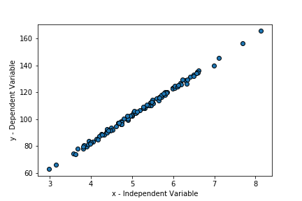
Based on the above figure, we can see that there is a clear linear relationship between x and y (What a strange coincidence)

Note. The numpy library has a host of linear algerbra functions (numpy.linalg)

Creating the A and B matracies

#Create column of ones (This is for the intercept)
col1 = np.ones((data.shape[0], 1)) 
#Create a numpy array from the x variable in the above pandas data frame
col2 = np.array(data.x)
#Create A
A = np.column_stack((col1, col2))
#Create B
B = np.array(data.y)

Perform the above mentioned matrix operations

#Left multiply A by A transpose
AtA = np.transpose(A) @ A
# Perform the explicit inverse on AtA
AtAinv = np.linalg.inv(AtA)

Before solving for x, let’s do a quick sanity check to see if the inverse was calculated correctly.

Remember that

\begin{equation}(A^{T}A)^{-1}(A^{T}A) = I \ Thus, (A^{T}A)^{-1}(A^{T}A)x = I x \end{equation}

print(AtAinv @ AtA)

[[1. 0.]
 [0. 1.]]

Solving for x

x = AtAinv @ (np.transpose(A) @ B)
print("a = ", x[0])
print("b1 = ", x[1])

a =  3.2436220896970553
b1 =  19.9273221320193

Let’s check our work by using sklearn

reg = LinearRegression().fit(A, B)
print("a = ", reg.intercept_)
print("b1 =", reg.coef_[1])

a =  3.2436220896965153
b1 = 19.927322132019434